Simplifying techniques for contour locating and Implementation on high-low centre labelling
Charles Luk (cluk19693@gmail.com)
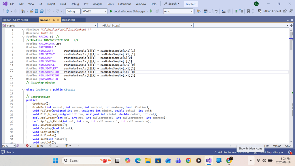
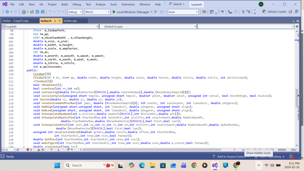
Update: The isobar.h screen print is added to the start of the Appendix A on 16 Feb 2026 for reference.
Update: A new posting on the full implementation of High Low labelling was released on 14 Feb 2026. With the addition of three paragraphs plus full details of C++ programming, Section B on High Low Labelling can be adapted to run on any contouring program.
Posting on 7th January 2026 :- The entire presentation in SECTION B on High-Low Labelling was completely revised.
First Posting date : 11 November 2025
The author is owner of the website : https://subtropicalrainstorms.ca/2026/03/17/a-study-of-200hpa-mid-latitude-disturbance-excitation-behind-a-12-hr-synoptic-scenario-on-imminent-extreme-rainstorm-occurrence-at-the-subtropical-region/
The presentation in the paper is largely programming-language-independent, except for the two Appendices, which, as extensions of the subject material, implement a walkthrough of Visual C++ program code compiled with Microsoft Visual Studio 2022.
The document, which offers an alternative approach to contour drawing by providing an algorithm for contour detection, linking, and ridge/trough center labeling, starts by converting a 2.5 ° latitude-longitude input grid to an x-y coordinate grid on a Mercator or Polar Stereographic projection. The next step subdivides the coarse row-column grid into a fine mesh grid through carrying out the following steps: 1) divide grid rows into sub-rows called raster, and down each column from the first to the last, interpolate from column-at-row intercepts into column-at-raster intercepts, and 2) divide grid columns into sub-columns, and across each raster from the top to the bottom, interpolate from raster-at-column intercepts into raster-at-sub-column intercepts. Dividing each fine mesh grid value by a contour interval at each grid point, a contour-interval-number integer field is obtained.
Introduction
In the nineteen-eighties, the contour linking method, which plays the crucial role in contour drawing, was based on a raster-cutting algorithm. By examining the grid point values on a raster, the contour-interval-number changes at successive columns are obtained. Each change location column is at a point of contour intersection on the raster. By arranging intersection locations from left to right on each raster before linking them pairwise from an upper raster to the next lower raster, contour segments between each raster pair are obtained. This method will not be discussed further here.
SECTION A. Contour Drawing
The method discussed was inspired by a University of Toronto Computer Science assignment on simulating water flow from an underground tunnel entrance to its exit. The simulation was generalized here to water flow which gushes from a hole on the ground anywhere inside an empty tunnel (with any number of entrances or exits), any irregularly shaped cave, or closed cavity (with no entrance or exit), each bounded by the wall, eventually reaches all areas of the continuous space.
In the first place, a swath of rasters is generated from the fine-mesh contour-interval-number integer field as a 2D floor plan of the cave. If at any grid (I,J) the contour-integer-number differs from that of its neighbor grid, it is on a contour which simulates a wall; otherwise, the grid (I,J) represents a white space on the floor plan. The 4 sides of the swathe rectangle represent the extent to which searching (simulating water flow) stops.
Simulation is performed by looping through a fine-mesh contour-interval-number integer field in the swath. At each(the primary) coordinate (I,J) where the grid value is not 255(which means the grid is unvisited), a global variable is set equal to the primary coordinate (I,J)’s value as the comparison target value for the search through the white space. A function call is made, passing the primary coordinate (I,J) as the parent parameter. Inside the function, the grid value at parameter (I,J) is compared against the global variable. If unequal (changing interval number), coordinate (I,J) is a contour intersection and should be appended to a contour intersection queue with immediate return to its call parent. If equal (remarks: inside the first level call by primary parent, the answer is always yes since it is a self comparison), it suggests coordinate (I,J) is in the continuous white space as its parent, and a function call to each neighbor coordinates (except the parent) is made by passing the its (I,J) as the test-location parameter and its own (I,J) as the referring-parent parameter. Because the function call becomes recursive, the result can generate an indefinite number of branches until every individual function returns on 1) encountering a contour intersection, 2) hitting the swathe boundary, or 3) arriving at a visited coordinate (I,J) whose value equals 255. In any case, all return calls made to the parent eventually converge to the primary parent.
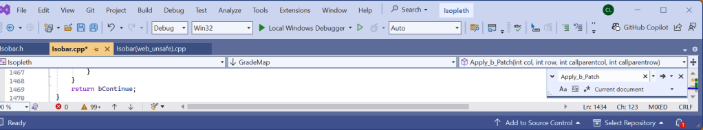
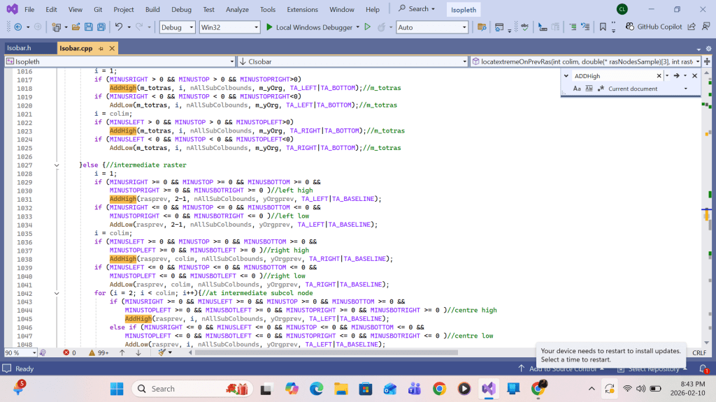
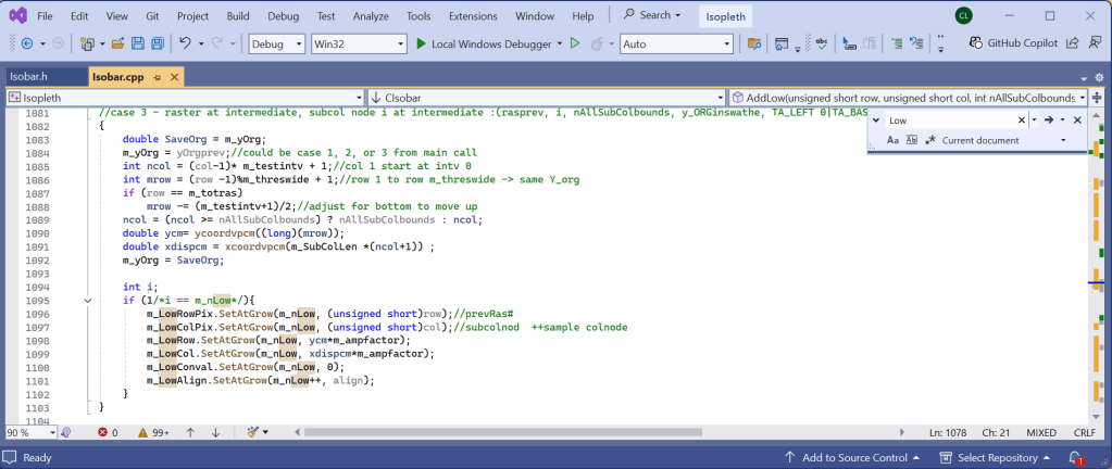
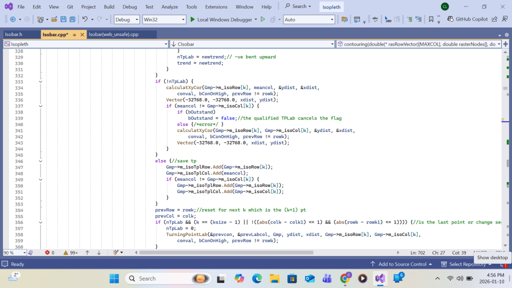
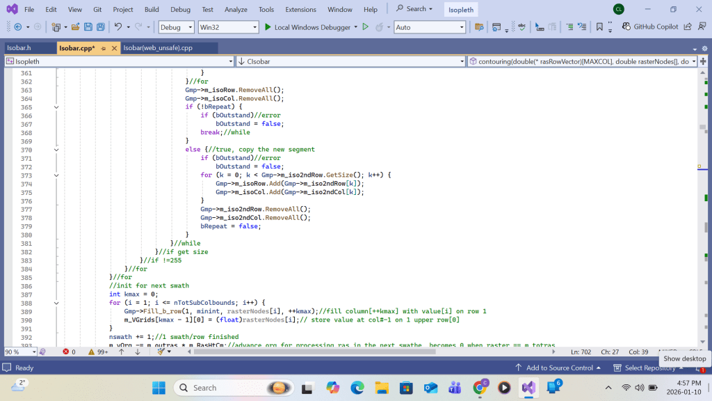
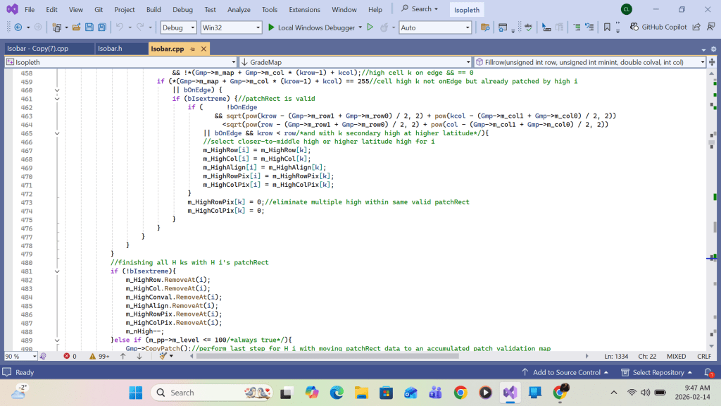
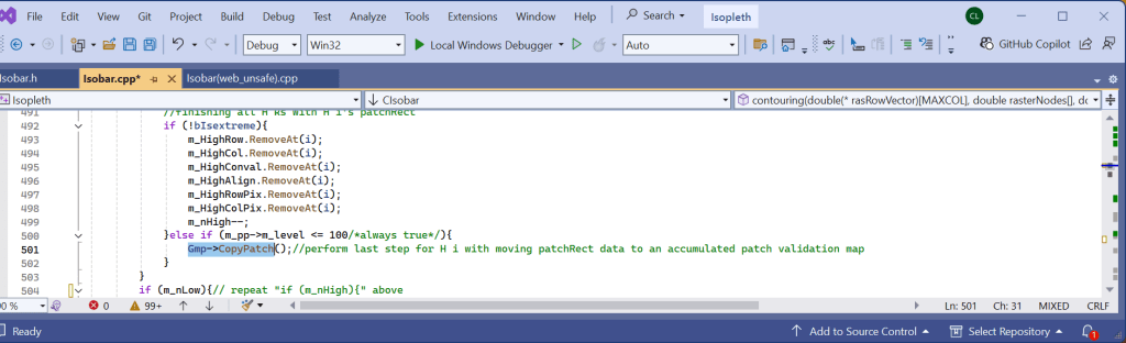
Following is a screen(1 and 1/2) shot copy of the recursive function:

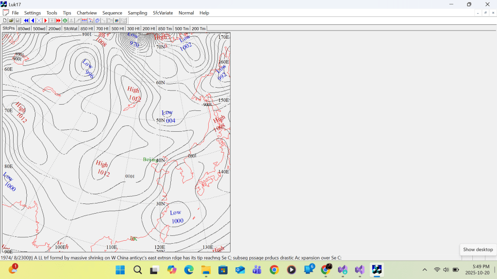
Function call made at each primary coordinate (I,J) will result in the detection and storage of contour coordinates in a queue. By linking these coordinates in proper sequence, all the contour lines drawn, which may or may not reach the top, left, right, or bottom of the swathe boundary, would enclose a continuous white space inside which the primary coordinate (I,J) lies. These contours may consist of contours with single or double contour-interval-integer values. Since contour intersections are encountered in a haphazard order during the search, the coordinates of different contour segments of equal or different contour-interval-integer values may occur in the queue in random order. If only reordering the segments without sorting intersection coordinates in the queue, the plotting result may end up in error, as shown in the next screenshot. First, broken or dotted contour lines would appear throughout the chart. Secondly, linking 2 contour intersections in the reverse direction, from right to left, would cause the contour label to be printed upside down, with an upward offset from the gap (refer to the top-left-hand corner of the chart).
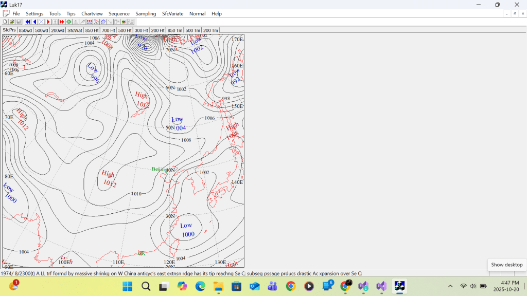
Below with sorting applied to the same case (which is tricky), the chart looks good.
SECTION: B. Maxima(High) and Minima(Low) Labeling
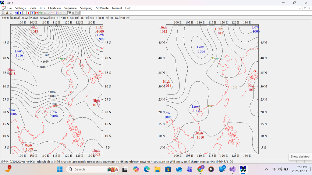
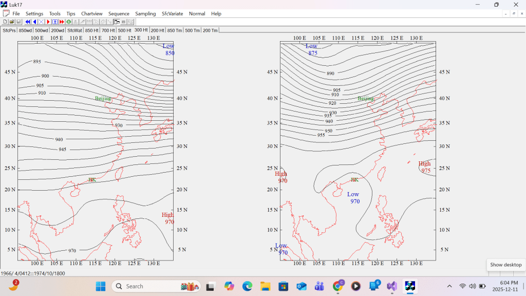
All centres of maxima (high or ridge inclusive) and minima (low or trough inclusive) can be located on the chart by simple comparison with surrounding field values. But in most cases, this would lead to duplicating max or min labels. The following shows two examples of duplicating labels.
First example MSL Pressure
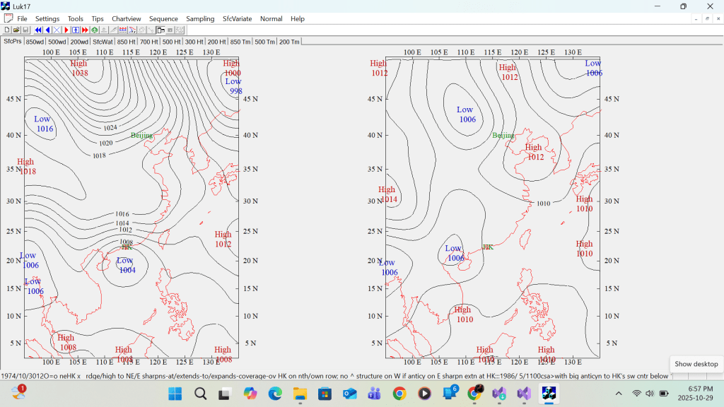
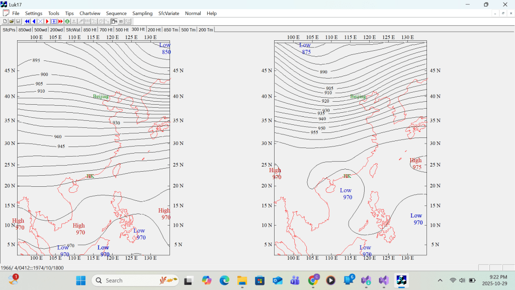
Second example 300 hPa contour height
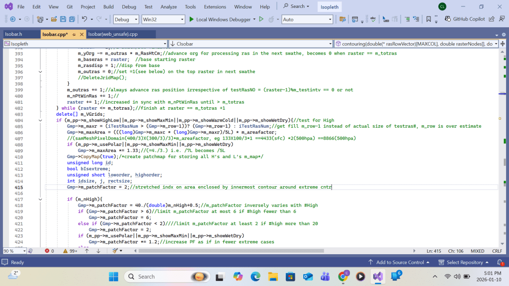
Apart from contour drawing, the recursive function approach for searching contour intersections in Section A can be applied to High/Low labeling. An integer grid field on contour interval number above( minus) a basic contour interval number is copied from the master grid (compilation* of which will be discussed later in this section) onto the integer grid m_map. Thus, the relationship of the m_map field’s grid value to the actual contour value equals
Actual integral contour value = (m_map field’s grid value + basic contour interval number) * contour interval width
The following discussion on High array applies to Low array. The construction* of the 2 arrays will be described later in this section. The array members of Highs are handled top-down. That means High array’s subscribe I loops from total#high to 2. After converting the H(i)’s contour(say MSL pressure) to its contour interval #, it is set equal to a global integer m_examGrade. The Recursive function is called by passing the H(i)’s row and column coordinates(i,j) as the test location parameters. The last argument ‘extype’ is set to +1 for H( as in this case) or -1 for L. Inside the function, the grid content at the test location parameter is compared with m_examGrade. If equal, the location content is set equal to 255. and the same function calls are made at the neighboring locations (coordinates). The succeeding locations will repeat the same process until a chart boundary is reached or a location’s content is not equal to m_examGrade. The function then relinquishes further neighbor calls and eventually backs up to the first parent. The result is a continuous grid domain with a grid value of 255. For each H(i), an inner High array with subscribe k loops from i-1 to 2. if a High array’s H(k)’s coordinates (i,j) on m_map is tested equal to 255, a duplication of H(i) occurring over the same domain is found, resulting the cancellation of either H(i) or H(k) from the list. After elimination duplication, the result of patching H(i) on m_map is then copied to grid m_patchmap by the function CopyPatch() for combining all individual High’s( and later Low’s) patch results for printing.
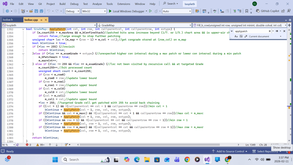
??
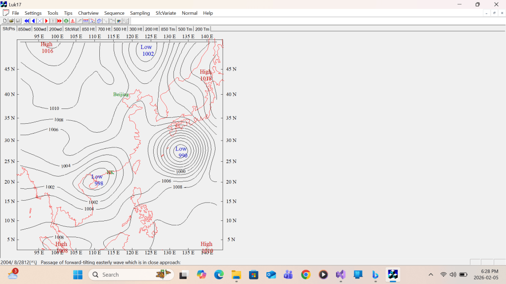
First example of corrected single H/L Labeling MSL Pressure
Second example of corrected single H/L Labeling 300 hPa contour height
Example of strong typhoon
Example of continental anticyclone in polar stereographic projection
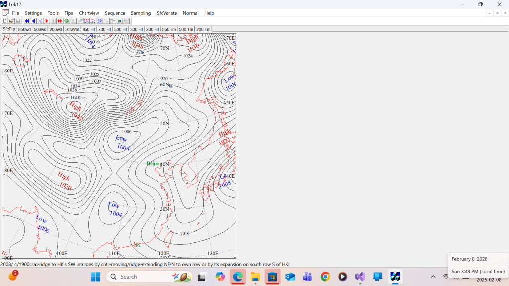
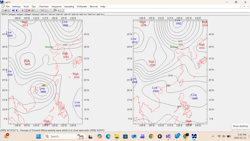
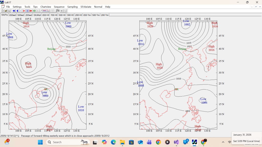
But this is not the end of story on label printing. Error in label printing does not only confine to duplicating labels over a single domain. The are 2 other common cases of mis-labeling. First, a col is an area or zone surrounded by high or low pressure areas. Therefore it shouldn’t be designated as a high pressure or low pressure area and hence should be label-free. Secondly very often, a low centre label which has no individual enclosing contour at the trailing end of anther deeper low is enclosed by the deeper low’s outer contour forming a complex low system. The same case occurs with some high centre label. This is superfluous as shown in the following example.
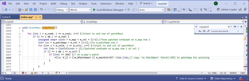
It has to be established that each label must be enclosed either by one closed contour or by broken single-value contour fragments with 1(up to 3) open endings on the chart edge boundary. Therefore, a label inside a col or complex H/L does not meet the single-value contour requirement. Any patch formed by calling the ApplyPatch() function on such a label should not be accepted in the subsequent CopyPatch() function call. But there is a simple solution. By introducing a global boolean variable ‘m_bPatchWarn’ in the GradeMap class and use it in the ApplyPatch() function, ‘m_bPatchWarn’ can be set equal to true for any single-value-contour violation in the course of building the patch. Inside the CopyPatch() function call, ‘m_bPatchWarn’ can be used to validate the resulting patch using the following check:
In Function CopyPatch(): *(loc + j) = (!m_bPatchwarn || m_warnCnt<4)? -Indx:Indx;// set patch result from ‘no PatchWarn flag or few m_warnCnt’ to -255 for printing.
The left example shows Highs labelled in the cols over the East China Sea and over Korea, an a complex Low over southwest China are removed. The right example shows the complex Lows across the western Pacific, the Philippines, and the South China Sea are reduced to a simple Low.
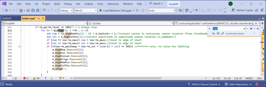
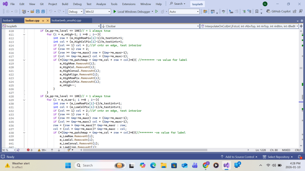
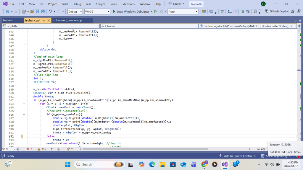
After all duplicated Highs/Lows in each 255 domain are eliminated, the coordinates of the unique Highs/Lows on m_patchmap can now be checked for validity using the following codes to apply necessary removal from printing.
With the addition of following three paragraphs plus full details of C++ programming, Section B on High Low Labelling can be adapted to run on any contouring program. We can start this by first exploring paragraph 1) the preparation of m_Master, which is the contour interval integer (low resolution) grid field derived(using horizontal row and vertical col sampling) from the floating point high resolution contour interval grid used for contour linking.
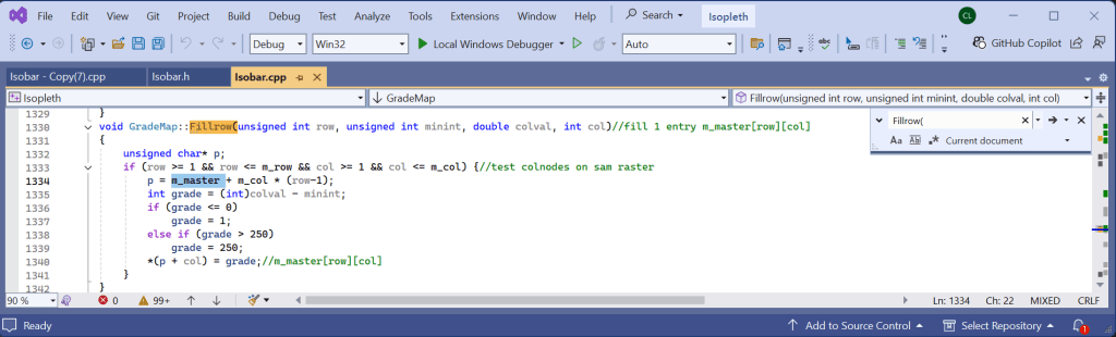
When looping through the rasters, the statement below fills 1 column entry of the m_master, the same entry is passed to the same column index at n_samNode on rasNodesSample[++n_samNode][2] = rasterNodes[j], which is also used for local Max/Min comparison in locatextremeOnPrevRas() displayed next.

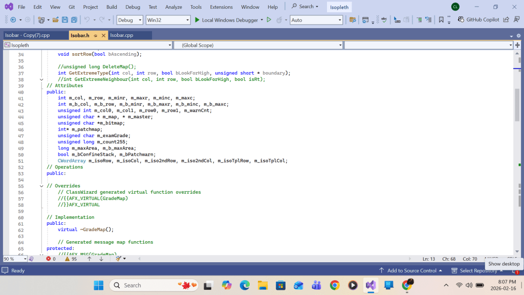
Paragraph 2) The building of the High/Low centres array is based on checking each grid point for local maxima/minima against its neighbouring 8 grid points. The following plain language terms used in the comparison statements can be referred to in the header file:


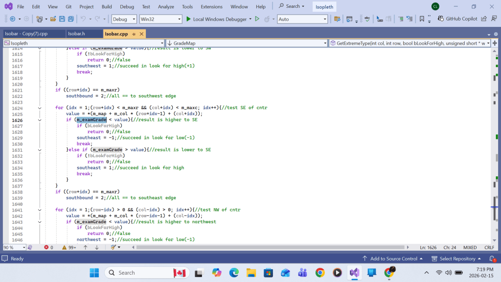
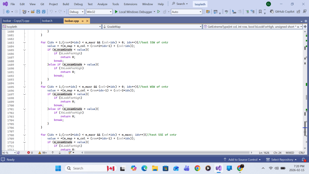
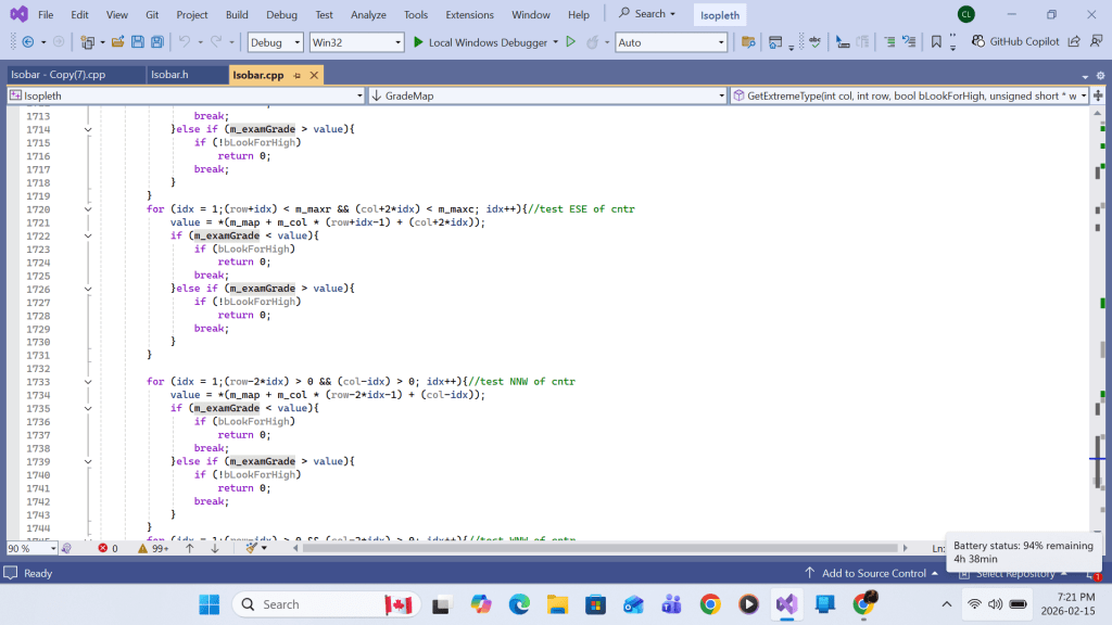
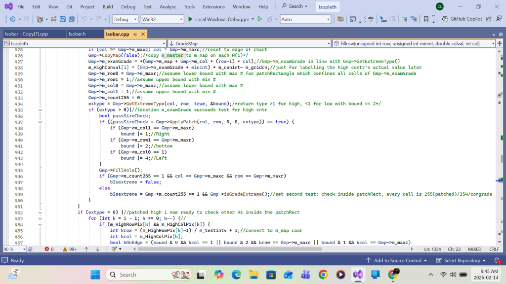
Paragraph 3) Call to ApplyPatch() for each high/low array member found in 2) should be preceded by call to a harsh validation function on high/low : int GradeMap ::GetExtremeType (int col, int row, bool bLookForHigh, unsigned short *westbottom). The function loops all 16-point compass directional distant from (row,col) by comparing them with the global variable m_examGrade until ‘break’ the loop either by hitting contour interval change or encountering chart boundary. It returns 1(high)/-1(low) for success in finding type or 0 in failure.


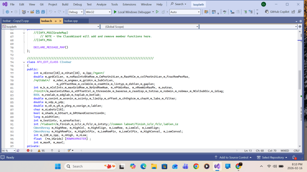
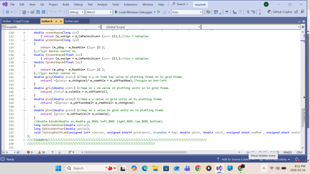
Appendix A: VC++ code for SECTION A on Contour Drawing (starting with isobar.h)
Summing up, upon return from the primary function Apply_b_Patch call at each grid(I,J), the following work will be completed for the white space area enclosing the primary grid: contour intersection queue sorting, queue elements’ contour-interval-number re-grouping, contour intersection retrieving/linking, and turning point labeling. Upon completing the loop over all grids (I,J), drawing all contour lines with turning point labels within the swathe area would be complete. Detailed implementation using Visual C++ code is shown in the screenshots that follow.

VC++ code for Appendix A for contour drawing ends here.
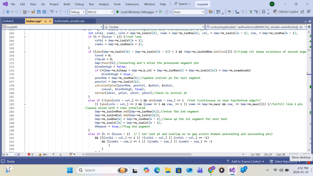
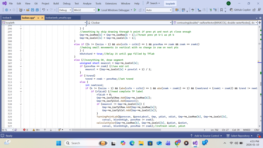
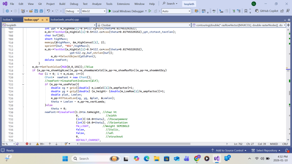
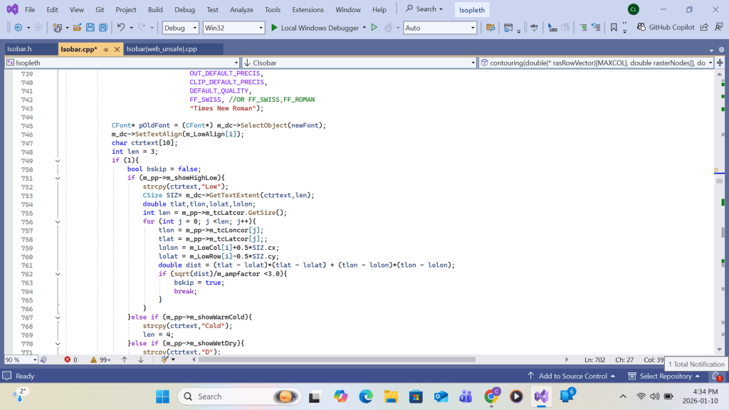
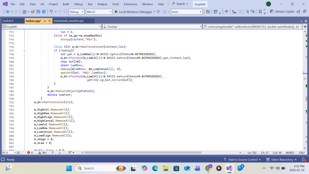
Appendix B: VC++ code in High, Low, Trough & Ridge Labeling
Listing for high-low labeling
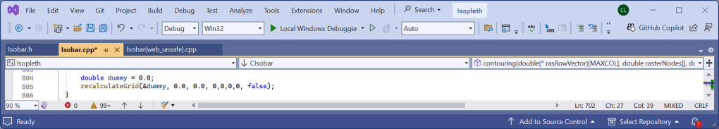
VC++ code for Low Labeling is similar to that of High Lebeling hence the Appendix B for VC++ code listing ends here. The program listing continues to show output-to-printer code.:

Acknowlegement
I gratefully acknowledge Met O 12(c) of the U.K. Meteorological Office for providing attachment training in the early 1980s under Mr Adrian Todkill and Mr P. Cockrell. The present work is derived from and substantially based upon an early version of CMAP developed by Met O 12. My contribution consisted of extending and adapting their framework through additional concepts and modifications, culminating in the development of my latest contouring program.
